The early generative model of restricted Boltzmann Machines and deep belief networks

The Hopfield network from the previous post is a very good librarian. Give it ten digits and it will return those ten digits from damaged copies. Ask it for an eleventh digit, one that looks like the others but was never stored, and it has nothing to offer. It remembers examples; it does not learn where the examples come from.

The Boltzmann machine closes that gap. Ackley, Hinton and Sejnowski introduced it in 1985 as a stochastic Hopfield network with two changes: the weights are learned so that the network's equilibrium distribution matches the data, and some neurons are hidden, free to represent structure that the pixels do not show directly. The result is one of the first generative neural models. Twenty years later, stacks of restricted Boltzmann machines trained one layer at a time were part of the work that made deep networks trainable again, which is a large part of why I wanted to implement them.

An energy over visible and hidden units

A restricted Boltzmann machine (RBM) has a visible layer v, which holds the data, and a hidden layer h. Units take the values 0 and 1 here, not ±1 as in the Hopfield network. The restriction is structural: there are connections between the layers but none inside a layer. The energy keeps the Hopfield form, with a bias for each unit:

double compute_energy() {
    // From Mehlig, p. 67
    energy = -visible.dot(weights * hidden) - visible.dot(b_v) - hidden.dot(b_h);
    return energy;
}

The missing intra-layer connections are what make the model practical. With the visible layer fixed, every hidden unit sees only visible units, so the hidden units are independent of each other. Each one switches on with a sigmoid probability of its local field:

The same holds in the other direction. A whole layer can therefore be sampled in one matrix product. sample_hidden does this for a batch of visible vectors stored as the columns of a matrix:

template <typename AggregateType>
void sample_hidden(const AggregateType& visible, AggregateType& hidden, bool do_sample,
    double temperature = 1.0) {
    // We stored the matrix w as a (visible, hidden) matrix so we need
    // to transpose w to compute the hidden local fields
    hidden_local_fields.noalias() = (weights.transpose() * visible).colwise() + b_h;
    auto& probs = hidden_local_fields;
    probs = (1.0 / (1.0 + (-hidden_local_fields.array() / temperature).exp())).matrix();
    if (do_sample)
        hidden = probs.unaryExpr([this](FloatingType p) {
            return (this->uni(this->rng) < p) ? FloatingType(1.0) : FloatingType(0);
        });
    else
        hidden = probs;
}

Two details are worth pointing out. The local-field buffers are members that are resized once per batch size, so the training loop does not allocate. The flag do_sample selects between a binary sample and the probabilities themselves, and the training loop uses both. Here the temperature divides the local field, so it is a true temperature: values below 1 make the units more decisive.

Learning is a difference of two correlations

We want the marginal distribution P(v) to put high probability on the training images. The gradient of the log-likelihood with respect to a weight has a compact form:

The first term is the Hebbian rule again: correlations measured with the data clamped on the visible layer. The second term is an anti-Hebbian correction: the same correlations when the network runs freely. Learning stops when the network, left alone, produces the same statistics as the data. The rule is local, because each weight needs only the activity of the two units it connects.

The difficulty is the second term. An exact model average needs the chain to reach equilibrium, which can take a very long time. Hinton's contrastive divergence (CD-k) replaces it with a short chain that starts at the data and runs for k steps. The chain has no time to reach equilibrium, but it moves in the direction in which the model distorts the data, and that is enough to give a useful gradient. This is the core of train_cd:

// This is the positive phase, DO  Sample the hidden states!
sample_hidden(batch_visible, batch_hidden, /* do_sample */ true);
// NOW we use CD-K to compute the negative phase.
negative_batch_hidden = batch_hidden;
sample_visible(negative_batch_visible, negative_batch_hidden, /* do sample */ false);
for (int cd_step = 0; cd_step < k; ++cd_step) {
    sample_hidden(negative_batch_visible, negative_batch_hidden, false);
    sample_visible(negative_batch_visible, negative_batch_hidden, /* do sample */ false);
}
sample_hidden(negative_batch_visible, negative_batch_hidden, false);
sample_visible(negative_batch_visible, negative_batch_hidden, /* do sample */ true);

weights += lr * (batch_visible * batch_hidden.transpose()) / batch_size;
b_v += lr * batch_visible.rowwise().mean();
b_h += lr * batch_hidden.rowwise().mean();
// negative phase
weights -= lr * (negative_batch_visible * negative_batch_hidden.transpose()) / batch_size;
b_v -= lr * negative_batch_visible.rowwise().mean();
b_h -= lr * negative_batch_hidden.rowwise().mean();
weights *= (1 - lr * decay);

The products batch_visible * batch_hidden.transpose() sum the outer products of the whole mini-batch in one call, which is where Eigen spends most of the training time. Mehlig presents the algorithm one pattern at a time; batching it changes nothing in the mathematics and a great deal in the speed.

The negative chain in this implementation passes probabilities between the layers and samples only the last visible state. This is a deliberate choice. It removes most of the sampling noise from the negative statistics, but it also turns the chain into a deterministic mean-field iteration instead of a true Gibbs sampler. Hinton's practical guide discusses which quantities in CD can safely be replaced by their probabilities; propagating them through all k steps is at the far end of that range. The last line applies a small weight decay, which keeps the weights from growing without limit.

Stacking machines into a deep belief network

One RBM learns one layer of features. To learn features of features, Hinton, Osindero and Teh stacked RBMs and trained them greedily: train the first machine on the images, map every image to its hidden probabilities, and use those as the training set of the next machine. StackedRBM::unsupervised_train implements that loop and swaps two dataset references between layers:

for (int machine_index = 0; machine_index < machines_stack.size(); ++machine_index) {
    auto& machine = machines_stack[machine_index].get();
    machine.train_cd(epochs, earlier, batch_size, lr, k, decay);
    // After each network is trained, the dataset is translated into its higher representation.
    if (machine_index < machines_stack.size() - 1)
        machine.map_into_hidden(earlier, later, batch_size);
    std::swap(earlier, later);
    later.clear();
}

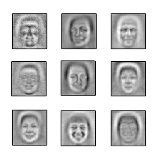
The current example trains a stack of three machines, 4,096 → 529 → 361 → 225 units, on 4,250 face images binarised to 64 × 64 with Niblack's method. Each layer gets 20 epochs with mini-batches of 125, a learning rate of 0.02 and k = 13. The same code also runs on binarised MNIST.

Seeing what a deeper layer sees

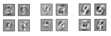
For the first machine, the column j of the weight matrix has one entry per pixel, so it can be displayed as an image: the pattern that hidden unit j responds to most. A unit in the second machine has no pixels; it is connected to the 529 hidden units below it. To show it, the code projects it back through the lower weights, which is a matrix product:

void compute_higher_order_kernels( Matrix& lower_semantic_weights, Matrix& out_location ) {
    // if this-> machine has weights ( hidden x hidden_upper ), the lower machine has
    // weights ( visible_before x hidden ): the product obtains hidden_upper kernels
    // of size visible_before
    out_location.noalias() = lower_semantic_weights * weights;
}

visualize_kernels_depthwise chains these products up the stack: W₀W₁ for the second layer, W₀W₁W₂ for the third. The projection ignores the sigmoids between the layers, so it is a linear approximation of what the deep unit prefers, not an exact preferred input. It is still a good picture of how the features change with depth.

Letting the machine generate

A Hopfield network given a random state falls into one of its stored memories. An RBM given a random state can produce something new that resembles the training data, because it models a distribution instead of a list of patterns. The example starts the first machine from sparse noise, with 15 % of the pixels on, and runs five steps of the chain at temperature 0.8:

BoltzmannLogger<float> logger;
logger.set_collect_states(true, "boltzmann_states.gif", MNIST_SIZE, MNIST_SIZE);
machine_0.attach_logger(&logger);
machine_0.random_visible(/* sparsity */ 0.15);
machine_0.run_cd_k(5, false, 0.8);

What the price was

The Boltzmann machine takes the Hopfield energy and turns it into a probability model with learned features, and the learning rule stays local and Hebbian at its core. The price is sampling. Every gradient step needs a Markov chain, and the quality of the gradient depends on how close that chain gets to equilibrium. Backpropagation in feed-forward networks later removed that cost and took over supervised learning, but the energy-based view survived in newer generative models.

Both models so far describe the data with an energy. The next post drops the energy completely. A Kohonen map learns with a different principle, competition between units arranged on a grid, and it gives something the RBM does not: a picture of the data in which similar inputs land next to each other.

References

- Ackley, D. H.; Hinton, G. E.; Sejnowski, T. J. (1985). “A learning algorithm for Boltzmann machines.” Cognitive Science 9(1), 147–169.
- Mehlig, Bernhard (2021). Machine Learning with Neural Networks: An Introduction for Scientists and Engineers. Cambridge University Press.
- Mehlig, Bernhard. Machine learning with neural networks, lecture notes, arXiv:1901.05639.
- Hinton, G. E. (2002). “Training products of experts by minimizing contrastive divergence.” Neural Computation 14(8), 1771–1800.
- Hinton, G. E. (2010). “A practical guide to training restricted Boltzmann machines.” UTML TR 2010-003, University of Toronto.
- Hinton, G. E.; Osindero, S.; Teh, Y.-W. (2006). “A fast learning algorithm for deep belief nets.” Neural Computation 18(7), 1527–1554.
- Niblack, W. (1986). An Introduction to Digital Image Processing. Prentice Hall.
- The Nobel Prize in Physics 2024: John J. Hopfield and Geoffrey E. Hinton.
- Zani, Lorenzo. associative-memory: a pure C++ learning resource for foundational machine learning. GitHub repository.