Hopfield Networks: an early model for reconstruction and associative memory

Show someone a torn photograph of a friend and they will still recognise the face. The missing half does not stop recall; it only makes it take a moment longer. In 1982 John Hopfield turned that observation into a physical system. In his network a memory is not a record that is looked up at an address. It is a state where the dynamics of the network comes to rest, and a damaged input rolls toward it the way a marble rolls to the bottom of a bowl.

This is the first post in a short series about associative-memory, a C++ repository where I implemented a few models that came before modern deep learning: Hopfield networks, Boltzmann machines, Kohonen maps and reservoir computers. Most of the ideas came from Bernhard Mehlig's Machine Learning with Neural Networks, which treats these models with the tools of statistical physics. I wanted to build them from the matrix products up, because each one isolates a single principle that later architectures absorbed.

The Hopfield network is the right place to start. It is small enough to hold in your head, it was one of the first neural models with a precise link to neuroscience and physics, and its ideas are still in use: the 2024 Nobel Prize in Physics went to Hopfield and Hinton for foundational work on machine learning with artificial neural networks, and "modern" Hopfield networks with continuous states have been shown to share their update rule with the attention mechanism of transformers.

Patterns are stored in the couplings

The network has N binary neurons with states s_i ∈ {−1, +1}. Every pair of neurons is connected by a symmetric weight w_ij. To store a set of patterns x^(μ), Hopfield used a rule that Donald Hebb had proposed for real synapses decades earlier: neurons that are active together strengthen their connection.

In matrix form, each new pattern adds its own outer product to the weight matrix. That is exactly what HebbianPolicy::store does. The pattern arrives as a packed BinaryState, is expanded into a ±1 vector, and is added as a rank-one update. The diagonal is cleared afterwards because a neuron must not reinforce itself.

virtual void store(BinaryState& bs) override {
    this->memorized_amt++;
    for (int i = 0; i < this->net_size; ++i)
        this->intermediate(i) = (bs.get(i)) ? DataType(1) : DataType(-1);
    // Note eigen optimizes this.
    this->weights.noalias() +=
        (this->intermediate * this->intermediate.transpose()) / this->net_size;
    this->weights.diagonal().setZero();
}

The weighting scheme is a template parameter of the network, so the compiler knows the concrete policy when it builds the update loop. The repository has three: the dense Hebbian rule above, the Storkey rule that we will meet later, and a matrix-free policy that recomputes each weight from the stored patterns. The matrix-free version trades time for memory, which matters when a 128 × 128 image gives a network of 16,384 neurons and a dense float matrix of about 1 GB.

Recall is a descent in energy

Storing patterns is only useful if the network can return to them. Each neuron looks at its local field, the weighted sum of the other neurons, and aligns with it:

Hopfield's key observation was that this rule minimises a quantity he called the energy (in this case, a negative quantity):

If one neuron changes sign, the energy changes by −2 |b_i| or not at all. Because the weights are symmetric and the diagonal is zero, the energy can never increase under one-neuron updates, and a finite network must stop at a local minimum. The stored patterns are such minima, provided there are not too many of them. The energy in the code is the same quadratic form:

virtual DataType energy(const BinaryState& bs) override {
    for (int i = 0; i < this->net_size; ++i)
        intermediate(i) = (bs.get(i)) ? 1 : -1;
    return -0.5 * intermediate.dot( weights * intermediate );
}

The guarantee depends on the order of the updates, so DenseHopfieldNetwork::run supports three policies. Asynchronous updates pick one random neuron per step and follow the argument above exactly. Synchronous updates change every neuron at once; they are fast with a single matrix–vector product, but they can oscillate between two states forever. Group updates sit between the two and change a random subset per step. This is the asynchronous branch:

else if (uc.up == UpdatePolicy::Asynchronous) {
    // Select a single state and act upon it.
    auto state_index = NetUtils::pick_random_state(this->network_size);
    update_indexes.push_back(state_index);
    this->policy.compute_local_fields(
        this->binary_state, update_indexes, local_fields_out);
    // Apply the signum activation function and notify.
    this->binary_state.set_value(state_index, MathOps::sgn(local_fields_out[0]) > 0);
    this->notify_state(std::tuple(state_index, this->binary_state.get(state_index)));
}

The notify_* calls feed a set of observers. A HopfieldLogger can collect the states into a GIF, and it can record the energy and the order parameters over time. The network computes those quantities only if a logger asks for them.

Denoising a handwritten five

The example stores one representative of each MNIST digit, binarised with Otsu's method, in a network of 784 neurons. It then takes the stored five, flips each pixel with probability 0.15, and lets the network run with groups of 60 neurons per step:

BinaryState deformed_5(MNIST_SIZE * MNIST_SIZE);
deformed_5.copy_content(binary_states[5]);
StateUtils::perturb_state(deformed_5, /* Noise level */ 0.15);

UpdateConfig uc = { UpdatePolicy::GroupUpdate, 60 };
dhn.feed(deformed_5);
dhn.run(/* Iterations */ 200, uc);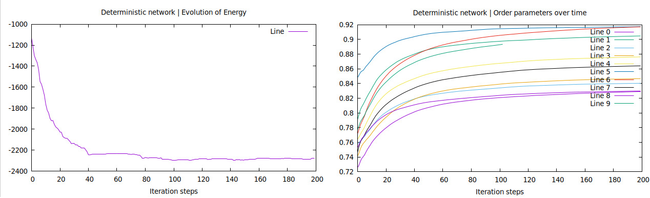

The energy curve shows the descent: most of the work happens in the first 40 steps, which is about 2,400 single-neuron updates, or three passes over the network. After that the state sits in a minimum.

The order parameters on the right are more interesting than they first look. Each curve is the fraction of pixels on which the network agrees with one stored digit, averaged over time. Mehlig uses the overlap m_μ = (1/N) ∑_i s_i x_i^(μ) instead; the two are related by agreement = (1 + m_μ)/2. All ten curves end between 0.82 and 0.92. The network does not agree with every digit; the digits agree with each other. Most of an MNIST image is background, so any two binarised digits already match on most pixels. That shared structure is the central weakness of the Hebbian rule, and it has a name.

Where memories interfere

Feed a stored pattern \(x^{(\nu)}\) into the network and expand its local field. One term comes from the pattern itself; the others come from every other stored pattern:

The second term is the cross-talk. Mehlig multiplies it by \(-x_i^{(\nu)}\) to get \(C_i\): if \(C_i > 1\), the cross-talk is strong enough to flip bit i of a perfect memory on the first update. For random, uncorrelated patterns the cross-talk behaves like Gaussian noise, and the network holds about 0.14 N patterns before recall collapses. Digits are not random, so the real limit is far lower. HebbianCrossTalkTermVisualizer computes \( C_i \) for every pixel so that we can see where the interference lands:

for (int i = 0; i < size; ++i) {
    sum_i = 0.0;
    for (BinaryState* mu : init) {
        BinaryState& x_mu = *mu;
        const signed char x_mu_i = x_mu.get(i) ? 1 : -1;
        for (int j = 0; j < size; ++j) {
            if (j == i)
                continue;
            const signed char x_mu_j = x_mu.get(j) ? 1 : -1;
            const signed char x_v_j = reference.get(j) ? 1 : -1;
            sum_i += x_mu_i * x_mu_j * x_v_j;
        }
    }
    sum_i /= -((double)(reference.get(i) ? 1 : -1)) * size;
    if (sum_i < 0.0) sum_i = 0.0;
    cross_talks[i] = sum_i;
}

Negative values help recall, so the visualiser clips them to zero and shows only the harmful part. The example measures the seven against the four and the nine, three digits that share a long diagonal stroke.

The Hebbian rule adds every pattern without regard for what is already stored. The Storkey rule, available as StorkeyPolicy, subtracts the local fields that the existing weights already produce for the new pattern. This lowers the interference between correlated patterns and raises the capacity while keeping the rule local and incremental.

Adding noise on purpose

Cross-talk has a second effect. Besides the stored patterns, the energy landscape contains spurious minima, such as mixtures of three memories, where a deterministic network can get stuck. The stochastic Hopfield network replaces the sign function with a probability:

At large β the network behaves like the deterministic one. At small β it moves almost at random, which lets it climb out of shallow minima. The implementation is a sigmoid and a uniform draw:

static double boltzmann_probability(DataType value, double temperature) {
    return 1 / (1 + std::exp(-2 * temperature * value));
}

signed char compute_value(DataType local_field, double temperature) {
    auto prob = boltzmann_probability(local_field, temperature);
    if (uniform(generator) < prob)
        return true;
    return false;
}

Note the convention: the scheduled value multiplies the local field, so it plays the role of the inverse temperature β, not of the temperature. A schedule that anneals the network, from noisy exploration to a clean final state, must therefore increase this value over time. The AnnealingScheduler hierarchy provides constant, linear and user-defined schedules.

A classifier made of attractors

If each stored digit is a valley, the valley that a new image falls into is a prediction. The example feeds 2,000 unseen MNIST digits to the network, runs five group updates of 15 neurons each, and asks a HopfieldClassifier which stored pattern the final state agrees with most. If the best agreement is below 0.7, the image is rejected. The result is a 10 × 11 confusion matrix whose last column counts the rejections.

Ten attractors cannot capture the variety of handwriting in MNIST, and the correlations that caused the cross-talk above also pull many images into the wrong valley. The classifier is not a competitive model. It is a direct way to see what an attractor landscape does to data it has never seen.

What carries forward

The Hopfield network recalls, but generalizing is much more difficult: it holds exactly the patterns we give it and nothing about the distribution they come from. The stochastic version already contains the missing piece. At finite β it samples states with probability proportional to e^−βH, so the energy defines a probability distribution. If we could learn the weights so that this distribution matches the data, and add neurons that the data never sees, the network would become a generative model. That model is the Boltzmann machine, and it is the subject of the next post.

References

- Hopfield, J. J. (1982). “Neural networks and physical systems with emergent collective computational abilities.” PNAS 79(8), 2554–2558.
- Mehlig, Bernhard (2021). Machine Learning with Neural Networks: An Introduction for Scientists and Engineers. Cambridge University Press.
- Mehlig, Bernhard. Machine learning with neural networks, lecture notes, arXiv:1901.05639.
- Hebb, D. O. (1949). The Organization of Behavior. Wiley.
- Amit, D. J.; Gutfreund, H.; Sompolinsky, H. (1985). “Storing infinite numbers of patterns in a spin-glass model of neural networks.” Physical Review Letters 55, 1530.
- Storkey, A. (1997). “Increasing the capacity of a Hopfield network without sacrificing functionality.” ICANN’97, Lecture Notes in Computer Science 1327.
- Ramsauer, H. et al. (2020). “Hopfield Networks is All You Need.” arXiv:2008.02217.
- The Nobel Prize in Physics 2024: John J. Hopfield and Geoffrey E. Hinton.
- Otsu, N. (1979). “A threshold selection method from gray-level histograms.” IEEE Transactions on Systems, Man, and Cybernetics 9(1), 62–66.
- LeCun, Y.; Bottou, L.; Bengio, Y.; Haffner, P. (1998). “Gradient-based learning applied to document recognition.” Proceedings of the IEEE 86(11). (MNIST)
- Zani, Lorenzo. associative-memory: a pure C++ learning resource for foundational machine learning. GitHub repository.