Reservoir Computing, or how to create deep temporal unsupervised embeddings

Drop a stone into a pond and the surface keeps a record of it for a while. The ripples mix with the ripples of the stone before, and a careful observer who looks at the surface at one moment can say something about the recent history of stones. The pond does not learn anything: it has rich dynamics and a memory that fades.

Reservoir computing takes that picture literally. The three models earlier in this series, Hopfield networks, Boltzmann machines and Kohonen maps, treat each input as a static vector. Signals such as an electrocardiogram only make sense over time, and the usual tool for them, a recurrent network trained by backpropagation through time, is hard to train: gradients that pass through many time steps tend to vanish or explode. Around 2001 and 2002, Herbert Jaeger (echo state networks) and Wolfgang Maass with colleagues (liquid state machines) arrived independently at the same way around the problem: build a large recurrent network at random, never train it, and train only a readout that looks at its state.

I find this the most surprising model in the repository. It moves almost all of the computation into a system that nobody optimised. Maass proposed it as a model of cortical microcircuits, and the same idea now runs on physical substrates such as optical and mechanical systems, because any medium with suitable dynamics can be the reservoir.

A random network that remembers

The reservoir has a state \(\textbf{r}(t)\) of \(N\) units, a fixed input matrix \(W_{in}\)and a fixed recurrent matrix \(W\). At each step it combines the previous state with the new input and applies a nonlinearity g:

Classical echo state networks use g = tanh. This implementation uses a ReLU. The input is set with feed and consumed by the next call to run, so steps without input let the reservoir evolve freely:

void run() {
    ReservoirState pre_activation;
    if (has_input)
        pre_activation = echo_weights * state + input_weights * input_state;
    else
        pre_activation = echo_weights * state;
    // RELU activation function
    state = pre_activation.array().cwiseMax(0.0f).matrix();
    // Delete the previous input, e.g. this is 1 time use only.
    has_input = false;
    notify_on_norm_change();
    notify_on_state_change();
}

The state is a matrix, not a vector: each column is an independent reservoir run. This lets a whole batch of sequences go through the same sparse–dense product at once.

For the readout to be useful, the state must depend on the recent input history and not on how the reservoir was started. Jaeger called this the echo state property. The usual rule of thumb is to scale W so that its spectral radius, the largest absolute value of its eigenvalues, is below 1. Near 1 the echoes last long; well below 1 they fade quickly; above 1 the dynamics can amplify themselves and forget the input.

Building the reservoir

initialize_echo_weights draws a sparse matrix in which each entry is non-zero with probability p and Gaussian with standard deviation 1/√N. It then estimates the spectral radius and rescales the matrix to the requested value:

for (int i = 0; i < state_dim; ++i)
    for (int j = 0; j < state_dim; ++j) {
        // Only put nonzero with probability sparsity
        if (unif(gen) < sparsity)
            triplets_vector.push_back(Trip(i, j, norm(gen)));
    }
echo_weights.setFromTriplets(triplets_vector.begin(), triplets_vector.end());
double current_radius = MathOps::sparse_power_method(echo_weights);
if (current_radius > 0)
    echo_weights *= (spectral_radius_desired / current_radius);
echo_weights.makeCompressed();

The estimate comes from the power method, which repeatedly multiplies a vector by the matrix and reads the eigenvalue from the Rayleigh quotient b^TWb:

for (int iter = 0; iter < max_iters; ++iter) {
    Vector Ab = A * b;
    double norm = Ab.norm();
    Ab /= norm;
    double lambda = Ab.dot(A * Ab);
    // Check convergence with step size criterion.
    if (std::abs(lambda - lambda_old) < tol) {
        return lambda;
    }
    b = Ab;
    lambda_old = lambda;
}
// If we reach here, we did not converge!
return lambda_old;

A note is important here: the power method converges when a single real eigenvalue dominates. For arbitrary matrices, this may never happen. This method is only a heuristic, which is why a guard breaks after a sufficient number of iterations.

We can visualize the norm of the internal reservoir state over time with a logger class. The example feeds a sine window once and lets the reservoir run freely for 20 steps:

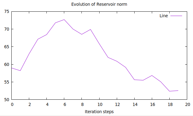
The norm starts at 59, rises to about 73 and is still at 52 after 20 steps. For large reservoirs where stability may be critical, an iterative method for non-symmetric matrices such as Arnoldi iteration, or the circular-law estimate σ√(Np) itself, gives a reliable value without forming the dense matrix.

Turning a heartbeat into a vector

The application is heartbeat classification on the MIT-BIH arrhythmia data, in a preprocessed form where each sample is one beat of 187 values with one of five labels: normal, supraventricular ectopic, ventricular ectopic, fusion and unknown. Reservoir::map cuts each beat into windows of 25 values, feeds the windows in order and keeps the final state as the embedding of the whole beat:

for (const auto& batch : input.batches(batch_size)) {
    // Reset the reservoir, setting the initial state to zero. This effectively begins a
    // new temporal sequence for the batches.
    reset();
    chunk.setZero();
    for (int c = 0; c < chunks_amt; ++c) {
        // The last chunk may be incomplete.
        const int start = c * input_dim;
        const int len = std::min(input_dim, dataset_input_size - start);
        for (size_t i = 0; i < batch.size(); ++i) {
            if (len < input_dim)
                chunk.col(i).setZero();
            chunk.col(i).head(len) = batch.x_of(i).segment(start, len);
        }
        run(chunk);
    }
    for (int i = 0; i < batch.size(); ++i) {
        output.add_sample(state.col(i), batch.y_of(i), batch.id_of(i));
    }
}

A beat of 187 values becomes eight steps of the reservoir: seven full windows and a last one with 12 values and 13 zeros. The reservoir has 625 units, so each beat ends up as a 625-dimensional vector that depends on the whole beat, with the most recent windows weighted most strongly. The state is reset for each batch of 1,000 beats, so no information leaks from one beat into the next.

Training only the readout

In a classical echo state network the readout is linear and is fitted in closed form by ridge regression. The repository uses a small multilayer perceptron instead, built on the same autograd module that the MLP example uses: 625 → 1,000 → 1,000 → 5 units, ReLU in the hidden layers and a softmax cross-entropy loss on the logits.

std::vector<int> units = { reservoir_size, N, N, 5 };
std::vector<ActivationFunction<float>> acts = { relu , relu, identity };
MultiLayerPerceptron<float> mlp(units, acts);

ScalarFunction loss_function;
auto y = loss_function.generator().create_vector_variable(5);
auto y_hat = loss_function.generator().create_vector_variable(5);
loss_function = loss_function.generator().smce_logits_true(y, y_hat);

It is trained on 15,000 embedded beats for 120 epochs, with mini-batches of 250 and a learning rate of 0.001, and it is checked on 3,000 beats that it never sees during training. The reservoir weights do not change at any point: the gradient stops at the embedding.

A description of the results is available in the repository discussion and in its example file.

Four principles, one repository

The reservoir finishes the series with the most extreme division of labour: a random dynamical system does the feature extraction, and learning touches only the last layer. It also shows why these older models are worth building by hand. A spectral radius is a single number in a configuration file, and it looks harmless, but whether the reservoir computes anything depends on how that number was obtained.

Across the four posts, each model isolated one idea. Hopfield networks store memories as minima of an energy. Boltzmann machines turn the energy into a probability model with hidden features. Kohonen maps let competition and cooperation build a topology. Reservoirs compute with fixed dynamics and a trained readout. Modern architectures mix all four ideas, with attention as a form of associative recall, energy-based and sampling-based generation, sparse competitive routing and fixed random features, and each of them is easier to see in the small model where it first appeared.

References

- Jaeger, H. (2001). “The ‘echo state’ approach to analysing and training recurrent neural networks.” GMD Report 148, German National Research Center for Information Technology.
- Maass, W.; Natschläger, T.; Markram, H. (2002). “Real-time computing without stable states: a new framework for neural computation based on perturbations.” Neural Computation 14(11), 2531–2560.
- Mehlig, Bernhard (2021). Machine Learning with Neural Networks: An Introduction for Scientists and Engineers. Cambridge University Press.
- Mehlig, Bernhard. Machine learning with neural networks, lecture notes, arXiv:1901.05639.
- Lukoševičius, M.; Jaeger, H. (2009). “Reservoir computing approaches to recurrent neural network training.” Computer Science Review 3(3), 127–149.
- Tanaka, G. et al. (2019). “Recent advances in physical reservoir computing: a review.” Neural Networks 115, 100–123.
- Tao, T.; Vu, V.; Krishnapur, M. (2010). “Random matrices: universality of ESDs and the circular law.” Annals of Probability 38(5), 2023–2065.
- Moody, G. B.; Mark, R. G. (2001). “The impact of the MIT-BIH Arrhythmia Database.” IEEE Engineering in Medicine and Biology Magazine 20(3), 45–50.
- MIT-BIH Arrhythmia Dataset (preprocessed), Kaggle.
- Zani, Lorenzo. associative-memory: a pure C++ learning resource for foundational machine learning. GitHub repository.