Self-organizing Kohonen Mappings for clustering and classification

Touch your thumb, then your index finger. The two sensations are processed by neighbouring patches of your somatosensory cortex, and the whole body is laid out across that strip of tissue in a distorted but continuous map. Vision and hearing have maps of the same kind: nearby points on the retina, and nearby frequencies in the cochlea, excite nearby neurons.

Teuvo Kohonen asked in 1982 what the simplest rule is that can make such maps form by themselves, without a teacher and without a genetic blueprint for every connection. His answer, the self-organising map (SOM), is the third model in this series. After the energy-based Hopfield networks and Boltzmann machines, it is interesting because it uses a different principle: units compete for each input, and the winner's neighbours on a grid learn with it. The outcome is a projection of high-dimensional data onto a two-dimensional sheet that keeps similar inputs close together.

The C++ class is called KonohenMapEigen, a letter swap that has stayed in the repository since the first commit. I will use Kohonen in the text and the real identifiers in the code.

Two spaces and one winner

A SOM connects two spaces. The input space holds the data, here 28 × 28 MNIST digits as vectors in ℝ⁷⁸⁴. The output space is a lattice of units, here a 10 × 10 grid. Each unit r has a weight vector w_r in the input space, a prototype of the inputs that it represents. For an input x, the best-matching unit is the one whose prototype is closest:

The weights are stored as the columns of one matrix, so the search for a single input is one Eigen expression:

unsigned int map(const Eigen::VectorXd& x) const {
    unsigned int winner = 0;
    (weight_vectors.colwise() - x).colwise().norm().minCoeff(&winner);
    return winner;
}

For a batch of inputs, the code avoids computing each difference by expanding the squared distance, \( ||x-w||^2 = ||w||^2 + ||x||^2 -2w^Tx\). The expensive part becomes a single matrix product between all prototypes and all inputs, which a BLAS-style kernel handles far better than a loop of subtractions:

Eigen::RowVectorXd w_norms = weight_vectors.colwise().squaredNorm();
Eigen::RowVectorXd x_norms = batch.colwise().squaredNorm();

Eigen::MatrixXd dist = w_norms.transpose().replicate(1, B)
    + x_norms.replicate(N, 1) - 2.0 * weight_vectors.transpose() * batch;

Eigen::VectorXi bmus(B);
for (int b = 0; b < B; ++b)
    dist.col(b).minCoeff(&bmus(b));

The neighbours learn with the winner

If only the winner learned, the SOM would be online k-means: every prototype would move toward its own inputs, and the grid positions would mean nothing. Kohonen's rule also moves the units that are near the winner on the grid, with a strength that decreases with lattice distance:

This cooperation is what builds the map. Two inputs that activate neighbouring units pull those units, and their neighbours, toward similar positions in the input space. Over many updates, units that are close on the grid end up with prototypes that are close in the data. The training loop in KonohenMapEigen::train is a direct translation:

for (const auto& input : data.get_data()) {
    // find best matching unit
    unsigned int bmu = map(input);
    int bmu_x = x_from_idx(bmu);
    int bmu_y = y_from_idx(bmu);
    // iterate over neighbors of BMU
    for (auto it = nf.begin(bmu_x, bmu_y); it != nf.end(bmu_x, bmu_y); ++it) {
        unsigned int idx = it.index();
        double h = it.contribution_weight();
        // update weights of neuron idx
        weight_vectors.col(idx) += learning_rate * h * (input - weight_vectors.col(idx));
    }
}

The neighbourhood is exposed as a forward iterator. NeighbouringFunctionEigen walks a square of radius support_size around the winner, clipped at the edges of the grid, and contribution_weight() returns the Gaussian Λ for the current unit. The training loop does not need to know whether the map is one- or two-dimensional.

The square support is an optimisation, and it has a visible effect. The example uses a support of 2, so at most a 5 × 5 block of units is updated. With the initial width σ = 3, the Gaussian is still 0.64 at the corners of that block. The effective neighbourhood at the start of training is therefore set by the square, not by σ.

Order first, then precision

A wide neighbourhood produces a global ordering, because the whole map moves together. A narrow one lets each unit specialise. Kohonen's practice is to start wide and shrink the width over time, and evolve_sigma provides four schedules. The exponential one is:

case exponential: this->sigma = sigma_0 * std::exp(-static_cast<double>(iteration_step) / tau);
    break;

The example uses \( \sigma_0=3, \tau=10 \) and a constant learning rate \(\eta=0.1\) over 100 passes through 4,000 digits. The width stays at 3 until pass 20. After that the schedule uses the absolute pass number, so at pass 21 \(\sigma\) drops at once to \(3e^{2.1} \approx 0.37\), and a direct neighbour of the winner then receives a weight of about 0.02. The training thus has two clear phases: 20 passes of ordering with a 5 × 5 neighbourhood, then 80 passes of what is almost pure competitive learning that refines each prototype in place.

Reading the map

The SOM is trained without labels, but we can use the labels afterwards to see what it learned. MajorityMappingEigen sends every training digit to its best-matching unit and counts the labels that each unit receives. A unit gets a label only if one digit makes up at least 60 % of its hits; otherwise it stays unlabelled.

int most_frequent_hit(int idx) {
    Eigen::VectorXd& labels = hits_map[idx];
    Eigen::Index maxIdx;
    int total = labels.sum();
    if (total == 0) return -1;
    float max = labels.maxCoeff(&maxIdx);
    if (max >= threshold * total) {
        return maxIdx;
    }
    return -1;
}

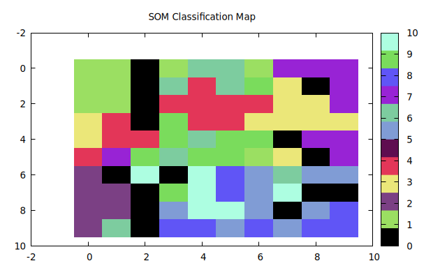
Units with the same label form connected patches, which is the topology preservation that the neighbourhood rule was designed to produce. The black units are as informative as the coloured ones. Several of them sit between two patches, where the prototype is a blend of two digits and no class reaches the threshold.

The labels are borrowed information. The map itself can also show its clusters, because the distance between neighbouring prototypes is small inside a cluster and large across a border. The U-matrix of Ultsch and Siemon makes this visible: for a W × H map it builds a (2W−1) × (2H−1) image in which the cells between units hold the distance between their prototypes and each unit cell holds the mean of its surroundings. UClusteringEigen::compute fills it like this:

if (x != width - 1) {
    float d_h = computing_distance(i, j);
    u(2 * x + 1, 2 * y) = d_h; // horizontal distance
}
if (y != heigth - 1) {
    float d_v = computing_distance(i, k);
    u(2 * x, 2 * y + 1) = d_v; // vertical distance
}
if ((x != width - 1) && (y != heigth - 1)) {
    float d_d = computing_distance(i, z);
    u(2 * x + 1, 2 * y + 1) = d_d; // diagonal distance
}
double value = neighb_mean(2 * x, 2 * y);
u(2 * x, 2 * y) = value;

The repository offers two more views: a full 100 × 100 matrix of distances between all prototypes, and k-means with ten clusters run on the prototypes instead of on the raw images. Because the prototypes are already an ordered summary of the data, k-means on 100 vectors is cheap, and its clusters can be drawn back onto the grid.

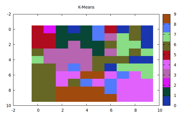
Compare this picture with the majority labels. k-means knows only prototype distances, but its clusters also form mostly connected regions on the grid. This is the practical value of a SOM: the grid is a coordinate system in which ordinary tools produce readable results.

Competition as a learning principle

The SOM update is a Hebbian-style rule: move the weights toward the input that activated the unit. On its own that rule would only average. Competition decides who learns, and the neighbourhood decides who learns with them. Those two additions are enough to turn a collection of prototypes into a map. The same winner-take-all idea reappears in vector quantisation and, in a different form, in the top-k routing of mixture-of-experts layers.

All three models so far see each input as a static vector. Real signals arrive over time, and a heartbeat or a sentence only makes sense as a sequence. The last post of the series turns to a model that computes with time itself: a large, random, fixed recurrent network whose only trained part is the readout.

References

- Kohonen, T. (1982). “Self-organized formation of topologically correct feature maps.” Biological Cybernetics 43, 59–69.
- Mehlig, Bernhard (2021). Machine Learning with Neural Networks: An Introduction for Scientists and Engineers. Cambridge University Press.
- Mehlig, Bernhard. Machine learning with neural networks, lecture notes, arXiv:1901.05639.
- Kohonen, T. (2001). Self-Organizing Maps, 3rd edition. Springer.
- Ultsch, A.; Siemon, H. P. (1990). “Kohonen’s self organizing feature maps for exploratory data analysis.” Proceedings of the International Neural Network Conference (INNC-90), Paris.
- LeCun, Y.; Bottou, L.; Bengio, Y.; Haffner, P. (1998). “Gradient-based learning applied to document recognition.” Proceedings of the IEEE 86(11). (MNIST)
- Zani, Lorenzo. associative-memory: a pure C++ learning resource for foundational machine learning. GitHub repository.